Just a quick post - there will be more on the way! Are you a student trying to work out what to study at university? Or someone just looking for something new to learn? Well, if so, then this could be just for you! MOOCs are becoming more and more popular and now the University of Southampton are offering one based in oceanography! From experience, I can tell you that oceanography is an incredible degree and you get to cover some truly interesting things! However, I was myself a little unsure about doing it when coming to university just because I had done so little of it before. This is why I think the MOOCs are a great opportunity to learn something new, and explore a discipline that, as a student you might not of covered much before. Also, let's remember that the oceans cover ~70% of the Earth's surface so they are pretty important!!!
Anyway, the course starts tomorrow (sorry, really should have posted this much earlier!) but it isn't too late to sign up.
This is the link for more information: https://www.futurelearn.com/courses/exploring-our-oceans
http://www.southampton.ac.uk/moocs/exploring_our_oceans.shtml
They are FREE and can be completed online, from the comfort of your own home! So, what is stopping you from signing up!
This is the link to follow their blog which, even if you aren't doing the course, should prove to be an interesting read anyway! http://moocs.southampton.ac.uk/oceans/
This is not the only Earth Science related MOOC out there (just google it and you will find loads!) and they are great ways of expanding your knowledge - let me know if you find any good ones! This is the only Oceanography based one I have found and there isn't really anywhere better to do it than with the National Oceanography Centre!
For those of you signed up, I hope you enjoy it and learn loads! The oceans are a truly fascinating thing yet so much remains unknown!
Showing posts with label Oceanography. Show all posts
Showing posts with label Oceanography. Show all posts
Sunday, 2 February 2014

Wednesday, 7 March 2012
Where would the British be without the Gulf Stream!?
Hello everyone! Hopefully everyone is enjoying the new climate module! Millie has written a very useful and succinct summary (something I never manage to achieve!) post on all the basics we have covered so far so there is no point me doing it to......instead I am going to write a little about the ocean circulation. After a polite reminder that Geography is the study of peoples interaction with the environment I am going to focus on the impact that the Gulf Stream has had on our development and the way society functions; projecting this into the future to examine how we would cope without it; rather than focusing on the science (although this is incredibly interesting, for the exam, unfortunaltely we do not seem to need to know that much - however feel free to ask lots of questions as this links with my EPQ topic).
I will get the sciency bit out of the way first....
I will get into trouble if I talk anymore about the theory but just a quick mention for the deep water circulation (just ignore the next paragraph if you don't want to know anything more than we strictly need to - the bit after is very relevant though)......
All the currents are linked in a complicated way and are dependent on each other. The sinking of Gulf Stream waters at high latitudes, feeds the crucial Thermohaline Cirulation (THC). Due to the combination of high evaporative salt enrichment
and Gulf Stream presence, THC is best developed in the Atlantic. The Gulf
Stream transports warm, salty water to the north-east of the Atlantic where it
cools, mixing with the cold Arctic Ocean waters. This causes it to become dense
enough to sink, both to the south and east of Greenland. The resulting current
is part of a larger system that connects the North Atlantic to the rest of the
Atlantic, Indian, Pacific and Southern Ocean, where the two main sinking
regions spread out in the subsurface ocean, thereby able to influence the
world’s oceans from depths of 1000m and below, before the cold, dense water gradually warms and returns to the
surface. Basically, the Global Conveyor Belt consists of surface and subsurface
currents, sinking regions and return waters which interlink to form a closed
loop. The conveyor starts in the Atlantic where salty water proceeds northwards
to Iceland, is thermally densified, and thus sinks through the interior to form
the conveyor’s lower limb. There are also deep-water flows such as the North Atlantic Deep Water (NADW), which have great influence on our lives. THC is very important. THC engages the
entire ocean into the climate system by permitting ocean water to directly
interact with the atmosphere (over a timescale of 100-1000
years), ergo, via the Gulf Stream and NADW, moderates the UK’s climate – one
that is, consequently, on average, 5°C
warmer than countries of similar latitude. On a more global scale, THC
influences biome distribution, NPP, sea level, ITCZ movement and productivity
of oceans whilst individual currents themselves allowed for the early
navigation of the oceans, thus aided development. However, the present pattern
has not always existed and is vulnerable to many external factors and cyclic atmospheric
changes. Even a significant weakening would have multiple detrimental impacts,
with the effects being globally experienced and, as the oceans control the
Earth’s climate over decades to centuries, understanding how they are likely to
change is crucial in selecting how to appropriately mitigate and adapt to
future climate change.
 Raises air temperatures, thereby helping to deliver mild winters and cool summers to the British Isles. The warmer waters have a significant impact on North Atlantic temperatures as they give up about one-third of the energy they had previously stored from the sun. The extent of the warmth provided by the Gulf Stream can be seen by comparing the climate of countries at a similar latitude to Britain's - i.e Canada which is a bit colder! It is believed that the UK climate is 5°C warmer than it would be without the Gulf Stream. Warming effect of Gulf Stream prescence enabled agricultral productivity to increase, permitting an acclerated transition through the early stages of the Rostow Model of Development.
 Sea level rise is potentially worrying for the UK as factoring in isostatic readjustment, population growth forcing more onto marginal lands and £130 billion worth of assets currently at risk of coastal flodding, greater than 10% as present, of our coastline would need to be protected. Even factoring in global climate change, the UK would still see reduced precipitation and 3C reduction in temperature. Increased snow cover would drastically decrease mobility, isolate people from an alrady straioned health care amongst other amenities, instigate higher living costs due to restrictions on agriculutre and issues with transporting food (in 2010 one milk company had to throw away 100,000 litres of milk) and cause huge disruption to education (altough, I don't think us students would mind a few more snow days!!!). Lower temperature and prolonged snow cover could cause issues for the UK's ageing population, with 1/4 in the southwest unable to heat their homes, possibly initiating greater urbanisation with cities able to offer facilities in close proximity, more likely to recieve greater funding for protection and the urban heat island effect warming, on average, summar and winter by 5C and 2C respectively. Consequently, a shift in employment could be experienced, with construction work becoming more seasonal and people looking for office-based work that can be completed from home during winter moths. Restricted agricultural and inducstrial productivity, fewer TNC's attracted whose presence stimulats cumulative causation and reduced touristic value, amongst other factors, is projected to generate a 2% reduction in the UK's GDP (-0.1% of global economy) with politicians put under increasing pressure to develop effective contingency plans to prevent societal collapse during protracted snow cover, minimise economci impacts and provide sufficient protection in coastal areas.
 The two hemispheres and the atmosphere and oceans are coupled in a way we don't need to understand but this means that, despite centralisation of impacts in the North Atlantic, impacts would be globally experienced. A 1C temperature increase in projected in the Southern Hemisphere, which would only be accentuated by global warming. A southward shift in the ITCZ would occur, reducing monsoon intensity/duration over India - worrying as India's water security is already poor, their rivers are reliant on glaciers, sea-level is threatening to displace millions thus increasing population density and India's population is expected to exceed China's by 2030. A 5% reduction in global NPP would be accompanied by alterations in temperate biome distribution and ecosystem disruption whilst with 20% of the world's fisheries dependent on upwelling systems and risng SST's futher reducing ocea oxygen content, food scarity would become prevalent especially with the global population soaring to 9 billion by 2045.
I will get the sciency bit out of the way first....
 |
This is a graphic I produced as part of my EPQ and so perhaps goes into a little two
much detail but the image in the top left hand corner illustrates really well the role of the
Gulf Stream in heat transfer
|
- Continents divide the oceans up into basins and so this complicates the direction of currents which are already inlfluenced by Coriolis in the same way as winds
- Gyres (large circular) form and move clockwise in the Northern Hemisphere
- Currents are driven by winds, Coriolis and the sinking of cool water near the Poles
- Antarctic Cirumpolar Current is the only current that goes right the way around Earth, preventing icebergs from entering the oceans - this is important when analysising possible threats capable of perturbing the ocean circulation
- Gulf Stream is initiated as water moves across the Atlantic from Africa to the Carribean. As it travels close to the Equator is gets heated. It then gets deflected by landmasses, Coriolis and other factors and so flows along the Florida coast. As it reaches higher latitudes it gets colder and saltier (we say salinity increases) as when ice forms, salt is removed from the fresh water and left behind in the ocean (brine rejection). This makes it more dense so it sinks.
- The Gulf Stream is a surface current but there are also other currents than flow deeper in the oceans. Together they connect all of the world's oceans, transporting heat, and forming the Global Conveyor Belt
 |
| Another graphic I made for my EPQ - atleast they are coming in handy! |
Why is the Gulf Stream important for the UK?
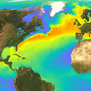 Raises air temperatures, thereby helping to deliver mild winters and cool summers to the British Isles. The warmer waters have a significant impact on North Atlantic temperatures as they give up about one-third of the energy they had previously stored from the sun. The extent of the warmth provided by the Gulf Stream can be seen by comparing the climate of countries at a similar latitude to Britain's - i.e Canada which is a bit colder! It is believed that the UK climate is 5°C warmer than it would be without the Gulf Stream. Warming effect of Gulf Stream prescence enabled agricultral productivity to increase, permitting an acclerated transition through the early stages of the Rostow Model of Development.
Perhaps the easiest way to understand the benefits of having the Gulf Stream nearby is to summarise the impacts on society if it was absent. Whilst there are many extrinsic forcing factors capable of shutdowning THC, thereby causing a southward shift or even complete shutdown of the Gulf Stream, the most likely is a large freshwater input at high latitudes due to melting ice, consequential to global climate change.........
How would the UK cope without the Gulf Stream?
This area is currently recieving a lot of attention (this is what I focused on when at the Met Office) and model simulations suggest that freshwater forcing of a shutdown, as a result of global climate change, could cause:
- 8C cooling
- Increase in wind speed
- Precipitation reduction
- Storms tending further north so hitting UK with increasing frequency
- 1-2 months additional snow cover
- 80cm sea level rise
- 2% reduction in the UK's GDP
 Sea level rise is potentially worrying for the UK as factoring in isostatic readjustment, population growth forcing more onto marginal lands and £130 billion worth of assets currently at risk of coastal flodding, greater than 10% as present, of our coastline would need to be protected. Even factoring in global climate change, the UK would still see reduced precipitation and 3C reduction in temperature. Increased snow cover would drastically decrease mobility, isolate people from an alrady straioned health care amongst other amenities, instigate higher living costs due to restrictions on agriculutre and issues with transporting food (in 2010 one milk company had to throw away 100,000 litres of milk) and cause huge disruption to education (altough, I don't think us students would mind a few more snow days!!!). Lower temperature and prolonged snow cover could cause issues for the UK's ageing population, with 1/4 in the southwest unable to heat their homes, possibly initiating greater urbanisation with cities able to offer facilities in close proximity, more likely to recieve greater funding for protection and the urban heat island effect warming, on average, summar and winter by 5C and 2C respectively. Consequently, a shift in employment could be experienced, with construction work becoming more seasonal and people looking for office-based work that can be completed from home during winter moths. Restricted agricultural and inducstrial productivity, fewer TNC's attracted whose presence stimulats cumulative causation and reduced touristic value, amongst other factors, is projected to generate a 2% reduction in the UK's GDP (-0.1% of global economy) with politicians put under increasing pressure to develop effective contingency plans to prevent societal collapse during protracted snow cover, minimise economci impacts and provide sufficient protection in coastal areas.
Global Impacts???
 The two hemispheres and the atmosphere and oceans are coupled in a way we don't need to understand but this means that, despite centralisation of impacts in the North Atlantic, impacts would be globally experienced. A 1C temperature increase in projected in the Southern Hemisphere, which would only be accentuated by global warming. A southward shift in the ITCZ would occur, reducing monsoon intensity/duration over India - worrying as India's water security is already poor, their rivers are reliant on glaciers, sea-level is threatening to displace millions thus increasing population density and India's population is expected to exceed China's by 2030. A 5% reduction in global NPP would be accompanied by alterations in temperate biome distribution and ecosystem disruption whilst with 20% of the world's fisheries dependent on upwelling systems and risng SST's futher reducing ocea oxygen content, food scarity would become prevalent especially with the global population soaring to 9 billion by 2045.
As you might have guessed, I find all of this stuff really interesting but I get the impression all you really need to know is the basic's of the Gulf Stream formation, a bit about how it has helped the UK and, just that society would struggle to sustain current livestyles without it - so hopefully this all made sense!
Friday, 23 September 2011
Geography Picture of the Week - Highest resolution global map of ocean surface salinity
First up, the most observant of you will notice that I have changed my 'Geography Picture of the Day' to 'Geography Picture of the Week' as, in reflection, it was always high unlikely that I would post a picture everyday! Instead, hopefully, I will be more likely to post one weekly and although I am guessing that most will be linked to physical geography, I will try and find some relevant to our current human module........
So, what is my Geography Picture of the Week this week???

The goal of the Aquarius mission is to retrieve salinity with a resolution of
0.2 parts per thousand (a concentration change equivalent to about one
millilitre of salt in six litres of water). Aquarius carries three high-precision radio receivers that will record the
natural microwave emissions coming up off the water's surface; emssions varying with the electrical conductivity of the water - a
property directly related to how much dissolved salt it is carrying.
The Nasa-Conae spacecraft is not the first ocean salinity mission in
orbit as Europe already have a satellite in operation (Smos) which was launched in 2009, producing the first ever global salinity maps generated from space. The intention is to inter-calibrate and combine the Aquarius and Smos
measurements as, together,these spacecraft are now acquiring volumes of salinity data that
dwarf all the information ever gathered in this field of study.
So, what is my Geography Picture of the Week this week???

I apologise to any of you who are getting fed up with oceanography-related posts (my EPQ will be over very soon so hopefully I won't be so tempted to write about oceanography stuff all the time when I should really be writing about Development and Globalisation!) but I really couldn't resist posting this one!!!
The above image was released by NASA and represents the one of the first and high resolution global map of ocean surface salinity made, using data acquired by the Aquarius/SAC-D satellite, launched in June this year with the map itself only incorporating the first 2 and 1/2 weeks of data since Aquarius became operational on the 25th August. Scientists have been able to measure ocean salinity for decades by lowering instruments from ships or by deploying robotic floats, but the technology to gather data from orbit is a recent innovation.
The generation of this map has been long anticpated by oceanographers and meterologists so I am guessing there are a few very happy scientists around the world at the moment! If you have followed any of my highly unorganised posts on oceanography you might be able to appreciate why........
Well, our ability to map and thus determine salinity (basically the 'saltiness') will improve our understanding of ocean circulation, the risks of future alterations to it and also an understanding of a few key climatic processes (note that the oceans and atmospheres are incredibly closely coupled with, in simple terms, the oceans provided the memory for the climatic signals generated in the atmosphere).
So, what excatly does this map show? Well, the red and yellow colours represent areas of high salinity with blues and purples denoting those with low salinity and black showing areas with no data(note no data retrival on land). The maps clearly shows well-established, large scale features, significantly the major salinity differences between the Atlantic, Pacific and Indian oceans. With the Pacific ocean by far the 'freshest', supporting the absence of deep-water formation sites, and the Atlantic by far the most saline. The salinity of ocean water is intrinsic to ocean circulation, although most precisely thermohalince circulation, which is soley driven by density differences (salty water is denser than less saline waters and so is forced to sink, thereby helping to drive the circulation). Also apparent is the corespondance between areas of lower salinity and rain belts and the areas of high evaporation found in the subtropics (regions of evaporative enrichment). Smaller-scale features are also possible to identify like the freshwater outflow from the Amazon River which acts to dilute immediate Atlantic surface waters.
 |
| Smos global salinity map |
Thursday, 15 September 2011
ENSO: a kind of synopsis
It looks like we are going to be doing a lot of purely Human Geography for a while and so, as well as writing a post about what I learnt about development this week I thought I would write a post on ENSO, a purely physical topic, that, if I am honest, really really fascinates me but is unfortunately no longer on the A-level syllabus. Just incase you don't manage to get to the bottom of this post, I am planning on writing up atleast one detailed case study that could be used in our essays (sorry to remind you all!) and so I am looking for some suggestions on which one to do - I have a few ideas but any suggestions would be greatly appreciated!
So, anyway, this one is for all you Physical Geographers out there!
What excatly is the El Nino Southern Oscillation (ENSO)?
 The term 'El Nino' has been applied, in the past, to somewhat different oceanographic events in the tropical Pacific but, nowadays, is commonly used to describe the anomalous warming of the sea-surface temperatures (SST) that occurs every few years in that region, although typically focused in east-central equatorial Pacific. El Nino events last several months and are associated with widespread changes in the climate system (dominating climatic flucuations observed on interannual timescales). These climatic changes have huge socio-economic impacts on countries, affecting agriculture, infrastructure, health, energy and, of course, development.
What is La Nina and the ENSO cycle?
La Nina is the term used to describe episodes of cooler than normal SST in the tropical Pacific (easiest way to think of it is the opposite of El Nino). The Southern Oscillation bit of ENSO is the term used for the atmospheric changes that occur in the tropical Pacific and accompany El Nino and La Nina events. Both events involve strong interactions between the oceans and atmosphere and tend to alternate (although not always the case) and this whole process is referred to as ENSO cycle. The ENSO cycle is not regular with various sizes and durations in both events but ENSO is a natural phenomenon and proxy evidence (principally from coral growth rate measurements) suggests ENSO has existed for thousands of years.

What causes El Nino?
As simply as I can put it, the ENSO cycle is the consequence of slow acting feedbacks in the ocean-atmosphere system, helped by strong air-sea interactions in the tropics that permit long-lived long-range connections to operate in the system.

Normally, the equatorial Pacific ocean has a pool of relatively warm water in the upper ocean to the west and a shallower layer of relatively cool water in the east; easterly surface winds are intrinsic to the maintainance of this balance. The first few tens of metres of oceans are well-mixed and lie above a thin thermocline, with cold water below.
The exact trigger of El Nino events is still debated and, due to a lack of observations, not a great deal can really be said about them with much certainity.There are a few possbile triggers though - Raised SSTs in central/east Pacific can be caused either through the action of westerly windbursts (short-lived storm-like events in West Pacific), or the gradual development of the ocean waveguide which moves the thermocline. Increased SST influences the atmospheric winds which, in turn, influence the upper ocean and the thermocline such that the SST is further increased = positive feedback. Only when the conditions are favourable will this feedback generate an El Nino event where you get increased SSTs, reduced easterly winds and a 'flatter' (for want of a better word) thermocline across east to west Pacific.
El Nino events then also cause gradual changes throughout the tropical Pacific ocan which develop in such a way that the SST across the equator slowly returns to normal, thus ending this event. However, the system normally overshoots and the feedbacks act to amplify small cooler anomalies, initiating a La Nina - as said before, it is basically the opposite with strengthened easterly winds and a increase in thermocline gradient. As this process is self-limiting the cycle continues....
What are the meteorological consequences?
If you have managed to stick with this to this point, this is probably the bit that will interest you the most - bringing in a bit of Human Geography you could even link this to the development essay as ENSO has, arguably, hindered development in countries across the world!
During El Nino events changes in SST, alterations to atmospheric circulation, temperature and precipitation occur; with these alterations, via atmospheric dynamics, extending far beyond the tropical Pacific region. As the impacts vary with location, it is practically impossible to identify a general pattern but generally speaking the eastward shift of precipitation in western Pacific tends to provoke huge deficits in the Philippines, Indonesia, north and east Australia, whilst central Pacific experiences increased rainfall.
I was fornutate enough to get to quiz an ENSO researcher at the Met Office, about everything related to ENSO and I saw lots and lots of similar maps to those opposite - one question that instantly came into my mind was why excatly do the maps suggest that ENSO has no impact whatsoever on Europe. Well, in short, the European region is only relatively weakly effects and there is substantial variability in the observed conditions. Therefore, only when you analysis a long historical record of events will you see the impacts. Such analysis suggests that there is a clear late winter response associated with moderate strength El Nino events; with the tendency for cold conditions in northern Europe and mild southern Europe, with an increased precipitation in a wide band across central Europe (accompanied by decreases elsewhere). Due to this though, it is hard to distinguish between the different factors, with El Nino just one, that are capable of generating such climatic anomalies.
What are El Nino 'flavours'?
I had never, ever heard of this idea of El Nino 'flavours' before and my knowledge is limited to what I am about to write (definetly requires a bit of further indepth research on my behalf!) but I thought I would mention it anyway as its quite an interesting idea. This topic has recieved quite a bit of attention in recent years, due to the slightly differing impacts. The 'normal' El Nino witnesses SST warming in eastern and central Pacific, while the 'dateline' or 'modoki' (apparently Japanese roughly translating to 'similar but different') type primarily experiences warming in the central equatorial Pacific. It has been suggested that the main difference is the influence in Atlantic tropical storms, with such storms typically fewer in 'normal' El Nino years, with 'modoki' events not reducing hurricane activity.
So, I think that is probably the basics of ENSO and I think, before I move on to talking about modelling it and how is it measured, I will probably have to write a post on the basics of climate modelling (it will be the real basics as all this modelling stuff is like a totally seperate science which I won't be able to tell anyone about in any great detail - trust me, its tricky stuff!) and, when I get my head around some scientific papers on ENSO the Met Office provided, I will also write a post on extrinsic forcing factors that effect ENSO. Just one last think to leave you with, follow the link to see up to date measurements taken in the Pacific as part of the Tropical Atmosphere Ocean project.
I am guessing that most are probably aware that we have just come out of a La Nina (cause of flooding earlier this year in Australia etc.) but at the moment scientists are divided over what will happen next as, although SSTs in Nino 3.4 started to rise again, they have since started to fall again - causing a split amongst researchers as to whether we will remain in the 'normal' state or go back into a La Nina (no one really seems to think we are going to go immediately into an El Nino). If you are interested and catch me around college, I have some plots, and ensemble forecasts which illustrate this.
I hope this made some sense (and was interesting), let me know if you didn't quite get everything as I realise that I am not great at explaining things but I am more than happy to try my best to explain it in a more understandable way if necessary. I am quite intrigued by the idea of El Nino 'flavours' and so if anyone knows anything more about it, please let me know!!! Especially things like what dictates whether an El Nino turns out to be of the 'normal' type or 'modiko' type?
There is some development stuff on the way, along with a few book reviews and a post primarily for all the new AS Geographers on 'Flooding, Farming and the Future'. Millie has emphasised the importance of knowing some case studies really well, with reference to development and colonialism, so I thought I would try and write a post on atleast one, sometime over the next few days, so let me know which one you would most like me to write about - its up to you!
So, anyway, this one is for all you Physical Geographers out there!
What excatly is the El Nino Southern Oscillation (ENSO)?
The term 'El Nino' has been applied, in the past, to somewhat different oceanographic events in the tropical Pacific but, nowadays, is commonly used to describe the anomalous warming of the sea-surface temperatures (SST) that occurs every few years in that region, although typically focused in east-central equatorial Pacific. El Nino events last several months and are associated with widespread changes in the climate system (dominating climatic flucuations observed on interannual timescales). These climatic changes have huge socio-economic impacts on countries, affecting agriculture, infrastructure, health, energy and, of course, development. What is La Nina and the ENSO cycle?
La Nina is the term used to describe episodes of cooler than normal SST in the tropical Pacific (easiest way to think of it is the opposite of El Nino). The Southern Oscillation bit of ENSO is the term used for the atmospheric changes that occur in the tropical Pacific and accompany El Nino and La Nina events. Both events involve strong interactions between the oceans and atmosphere and tend to alternate (although not always the case) and this whole process is referred to as ENSO cycle. The ENSO cycle is not regular with various sizes and durations in both events but ENSO is a natural phenomenon and proxy evidence (principally from coral growth rate measurements) suggests ENSO has existed for thousands of years.

What causes El Nino?
As simply as I can put it, the ENSO cycle is the consequence of slow acting feedbacks in the ocean-atmosphere system, helped by strong air-sea interactions in the tropics that permit long-lived long-range connections to operate in the system.
Normally, the equatorial Pacific ocean has a pool of relatively warm water in the upper ocean to the west and a shallower layer of relatively cool water in the east; easterly surface winds are intrinsic to the maintainance of this balance. The first few tens of metres of oceans are well-mixed and lie above a thin thermocline, with cold water below.
The exact trigger of El Nino events is still debated and, due to a lack of observations, not a great deal can really be said about them with much certainity.There are a few possbile triggers though - Raised SSTs in central/east Pacific can be caused either through the action of westerly windbursts (short-lived storm-like events in West Pacific), or the gradual development of the ocean waveguide which moves the thermocline. Increased SST influences the atmospheric winds which, in turn, influence the upper ocean and the thermocline such that the SST is further increased = positive feedback. Only when the conditions are favourable will this feedback generate an El Nino event where you get increased SSTs, reduced easterly winds and a 'flatter' (for want of a better word) thermocline across east to west Pacific.
 |
| La Nina |
El Nino events then also cause gradual changes throughout the tropical Pacific ocan which develop in such a way that the SST across the equator slowly returns to normal, thus ending this event. However, the system normally overshoots and the feedbacks act to amplify small cooler anomalies, initiating a La Nina - as said before, it is basically the opposite with strengthened easterly winds and a increase in thermocline gradient. As this process is self-limiting the cycle continues....
What are the meteorological consequences?
 |
| Global impacts of El Nino |
During El Nino events changes in SST, alterations to atmospheric circulation, temperature and precipitation occur; with these alterations, via atmospheric dynamics, extending far beyond the tropical Pacific region. As the impacts vary with location, it is practically impossible to identify a general pattern but generally speaking the eastward shift of precipitation in western Pacific tends to provoke huge deficits in the Philippines, Indonesia, north and east Australia, whilst central Pacific experiences increased rainfall.
 |
| Global Impacts of La Nina |
What are El Nino 'flavours'?
I had never, ever heard of this idea of El Nino 'flavours' before and my knowledge is limited to what I am about to write (definetly requires a bit of further indepth research on my behalf!) but I thought I would mention it anyway as its quite an interesting idea. This topic has recieved quite a bit of attention in recent years, due to the slightly differing impacts. The 'normal' El Nino witnesses SST warming in eastern and central Pacific, while the 'dateline' or 'modoki' (apparently Japanese roughly translating to 'similar but different') type primarily experiences warming in the central equatorial Pacific. It has been suggested that the main difference is the influence in Atlantic tropical storms, with such storms typically fewer in 'normal' El Nino years, with 'modoki' events not reducing hurricane activity.
So, I think that is probably the basics of ENSO and I think, before I move on to talking about modelling it and how is it measured, I will probably have to write a post on the basics of climate modelling (it will be the real basics as all this modelling stuff is like a totally seperate science which I won't be able to tell anyone about in any great detail - trust me, its tricky stuff!) and, when I get my head around some scientific papers on ENSO the Met Office provided, I will also write a post on extrinsic forcing factors that effect ENSO. Just one last think to leave you with, follow the link to see up to date measurements taken in the Pacific as part of the Tropical Atmosphere Ocean project.
 |
| Taken yesterday (14/09/2011) |
I hope this made some sense (and was interesting), let me know if you didn't quite get everything as I realise that I am not great at explaining things but I am more than happy to try my best to explain it in a more understandable way if necessary. I am quite intrigued by the idea of El Nino 'flavours' and so if anyone knows anything more about it, please let me know!!! Especially things like what dictates whether an El Nino turns out to be of the 'normal' type or 'modiko' type?
There is some development stuff on the way, along with a few book reviews and a post primarily for all the new AS Geographers on 'Flooding, Farming and the Future'. Millie has emphasised the importance of knowing some case studies really well, with reference to development and colonialism, so I thought I would try and write a post on atleast one, sometime over the next few days, so let me know which one you would most like me to write about - its up to you!
Friday, 2 September 2011
Met Office Work Experience - Day 5 (for 25-08-2011)
I realise that these posts on what I did at the Met Office are like a week late but I thought that, because I had such a great time and learnt an incredible amount, I would still write them! Well, what did I get up to on my last day with the Met Office?
 First up was a very interesting discussion with a researcher about ice sheets. There is currently a lot of uncertainity about ice sheets and their stability, with much of this uncertainity stemming from a lack of understanding of the mechanisms for ice sheet melt. Currently, it is believed that Antarctica is the most likely to experience significant melt and this is because much of it is under the sea. If the proportion that lies below sea-level was to melt, which scientists think could occur over the next few hundred years (although this may sound quite slow, it is considered to be rather rapid!), it would raise global sea-level by 6 metres!!! Greenland melting is an area that often recieves much attention, perhaps becuase we are unsure just how much freshwater could be released or how quicly it would occur, but for now alteast, many feel that a large freshwater input is unlikely. Before this discussion, I had never really given much thought to the influence that the angle of the bedrock, upon which the ice sheet lies, on melting but it does, in fact, seem to play quite a large role. The bedrock that the Greenland ice sheet lies upon slopes away from the sea, whilst that in Antarctica slopes towards the sea and thus making runaway melting possible. When the Laurentide Ice Sheet existed it was sat upon 'flat' bedrock, something that many considered essential for the occurence of Heinrich events. Due to this, depsite the fact that models currently cannot replicate Heinrich events, it is believed that this current climatic state cannot provoke Heinrich events. The fact that surprised me the most was that increased surface air or sea surface temperatures, as a result of global climate change, are not the biggest threat to the stability of ice sheets and would not be responsible for instigating the greatest volume of melt. Instead it is increased wind speeds.....but why?
 Well, increased wind speeds would raise the height of local sea-level and increase Ekman Pumping. Increased Ekman Pumping would provoke old warm waters from the deep ocean to be dragged closer to the surface and over the terminal morraine, which marks the end of glaciers or ice sheets, and towards the base of the ice sheet, thus causing melting to occur. This is believed to be responsible for more melting than raised surface air/sea temperatures. One thing that scientists are unsure of though is what happens to the warm water once it passes the terminal morraine. Does it hit the base of the ice sheet and then continually circle, gradually melting away the base or does it bounce back off and return to the rest of the ocean? Understanding this is, again, crucial if predictions of ice sheet melt are to become more cetain.....
Anyway, all of this 'stuff' is important if scientists are to make more certain predictions of the future of the MOC and there is a lot of debate over just how much of an impact melt of Greenland or Antarctica would have. Most focus is placed on Greenland, as a result of its location. Some feel that perhaps, if enough of Greenland melted, it could significantly reduce the MOC intensity whilst others believe that, due to existance of sinking sites either side of Greenland, that Greenland melt could provoke a switch in sinking sites to the western side of Greenland - a switch that could have the potential to actually warm the UK during winter. There are a couple of other quite specific topics that we covered but I think I will leave them for another blog post.
After this I attended a Modelling Team meeting which was quite interesting as it provided an insight into some of the work that researchers at the Met Office are currently doing and some of the problems they are facing at present. Following this I had a chat with someone regarding ENSO, a topic that fascinates me, and as, again, there was lots that we covered,and I am a bit more confident about talking about ENSO, I am going to write another post solely on this. The afternoon was finished off with a chat about the relationship between the ocean and atmosphere and how this relationship is replicated in models. The relationship between the ocean and atmosphere is really really complex and I literally touched the very very basics. The ocean is sort of like the memory of the Earth climate system. The atmosphere cannot store things, like signals or changes in climate, and so instead it passes the signals on to the oceans. The oceans can store this information for hundreds and hundreds of years, whilst it circulates them around the world, and then passes the signal back to the atmosphere where it provokes a short term, but rapid, response. This coupling is crucial for many things such as ENSO. It is tricky to model all of the processes that link the oceans and atmosphere and all of the exchanges that happen between them (I am in the process of writing a post on the real basics of climate modelling as it is like a whole new science).
I apologise as I realise that all of my posts regarding my time at the Met Office have been a bit all over the place but I honestly learnt so much and I am not that great at explaining things. Despite this, I still hope they have been interesting to read and have given you a bit of an insight into the work done at the Met Office and some of the things I was fortunate to do whilst up there. I really cannot thank the people who made this whole experience possible enough - I learnt an unbelievable amount, gained some invaluable advice universities courses and careers etc, got to meet some great and highly intelligent people and simply had just an amazing time!!!
First up was a very interesting discussion with a researcher about ice sheets. There is currently a lot of uncertainity about ice sheets and their stability, with much of this uncertainity stemming from a lack of understanding of the mechanisms for ice sheet melt. Currently, it is believed that Antarctica is the most likely to experience significant melt and this is because much of it is under the sea. If the proportion that lies below sea-level was to melt, which scientists think could occur over the next few hundred years (although this may sound quite slow, it is considered to be rather rapid!), it would raise global sea-level by 6 metres!!! Greenland melting is an area that often recieves much attention, perhaps becuase we are unsure just how much freshwater could be released or how quicly it would occur, but for now alteast, many feel that a large freshwater input is unlikely. Before this discussion, I had never really given much thought to the influence that the angle of the bedrock, upon which the ice sheet lies, on melting but it does, in fact, seem to play quite a large role. The bedrock that the Greenland ice sheet lies upon slopes away from the sea, whilst that in Antarctica slopes towards the sea and thus making runaway melting possible. When the Laurentide Ice Sheet existed it was sat upon 'flat' bedrock, something that many considered essential for the occurence of Heinrich events. Due to this, depsite the fact that models currently cannot replicate Heinrich events, it is believed that this current climatic state cannot provoke Heinrich events. The fact that surprised me the most was that increased surface air or sea surface temperatures, as a result of global climate change, are not the biggest threat to the stability of ice sheets and would not be responsible for instigating the greatest volume of melt. Instead it is increased wind speeds.....but why?  |
| This is a bit of an exaggeration of what happens but hopefully you get the general idea.... |
 Well, increased wind speeds would raise the height of local sea-level and increase Ekman Pumping. Increased Ekman Pumping would provoke old warm waters from the deep ocean to be dragged closer to the surface and over the terminal morraine, which marks the end of glaciers or ice sheets, and towards the base of the ice sheet, thus causing melting to occur. This is believed to be responsible for more melting than raised surface air/sea temperatures. One thing that scientists are unsure of though is what happens to the warm water once it passes the terminal morraine. Does it hit the base of the ice sheet and then continually circle, gradually melting away the base or does it bounce back off and return to the rest of the ocean? Understanding this is, again, crucial if predictions of ice sheet melt are to become more cetain.....
 Anyway, all of this 'stuff' is important if scientists are to make more certain predictions of the future of the MOC and there is a lot of debate over just how much of an impact melt of Greenland or Antarctica would have. Most focus is placed on Greenland, as a result of its location. Some feel that perhaps, if enough of Greenland melted, it could significantly reduce the MOC intensity whilst others believe that, due to existance of sinking sites either side of Greenland, that Greenland melt could provoke a switch in sinking sites to the western side of Greenland - a switch that could have the potential to actually warm the UK during winter. There are a couple of other quite specific topics that we covered but I think I will leave them for another blog post.
After this I attended a Modelling Team meeting which was quite interesting as it provided an insight into some of the work that researchers at the Met Office are currently doing and some of the problems they are facing at present. Following this I had a chat with someone regarding ENSO, a topic that fascinates me, and as, again, there was lots that we covered,and I am a bit more confident about talking about ENSO, I am going to write another post solely on this. The afternoon was finished off with a chat about the relationship between the ocean and atmosphere and how this relationship is replicated in models. The relationship between the ocean and atmosphere is really really complex and I literally touched the very very basics. The ocean is sort of like the memory of the Earth climate system. The atmosphere cannot store things, like signals or changes in climate, and so instead it passes the signals on to the oceans. The oceans can store this information for hundreds and hundreds of years, whilst it circulates them around the world, and then passes the signal back to the atmosphere where it provokes a short term, but rapid, response. This coupling is crucial for many things such as ENSO. It is tricky to model all of the processes that link the oceans and atmosphere and all of the exchanges that happen between them (I am in the process of writing a post on the real basics of climate modelling as it is like a whole new science).
I apologise as I realise that all of my posts regarding my time at the Met Office have been a bit all over the place but I honestly learnt so much and I am not that great at explaining things. Despite this, I still hope they have been interesting to read and have given you a bit of an insight into the work done at the Met Office and some of the things I was fortunate to do whilst up there. I really cannot thank the people who made this whole experience possible enough - I learnt an unbelievable amount, gained some invaluable advice universities courses and careers etc, got to meet some great and highly intelligent people and simply had just an amazing time!!!
Thursday, 1 September 2011
Met Office Work Experience - Day 4 (for 24-08-2011)
Last week I was fortunate enough to go back to the Met Office for a few more days and, yet again, I learnt so much, so I thought I would try and briefly go over some of the stuff I learnt. So, what did I get up to on Wednesday (I should probably say us as Millie also came along for the day!).......
Well, first up was a discussion about a possible thermohaline circulation shutdown. I have to admit that I find the idea of a future THC shutdown really interesting and it is an area that I have given a lot of thought to over the past few weeks, hence my rather long list of questions (I am guessing Millie quite enjoyed the fact that, for once, she wasn't the one my list of questions were aimed at!). As with the previous discussion groups we covered an awful lot so I am going to try and summarise the key points - feel free to ask if you want to know more! Again, much of the discussion revolved around the idea of hysteresis (which refers to the dependence of the state of a system on the history of its state, with the lag in a variable property of a system with respect to the effect producing it as this effect varies - thats kind of the idea of it all, I think). Honestly all of this takes a lot of time to get used to..... trust me I have been trying since we first started our EPQ's and I am, perhaps, only just starting to make some real progress!
I realise that I have spoken a bit about this graph before but, what excatly are the key points to take from it? Firstly, that a freshwater input does have the ability to weaken the THC and that a reduction in the freshwater present is crucial to a re-initiation of the THC. Secondly, that the THC seems to have two stable states; a stable 'off' and a stable 'on' state; and that, because of this, the same volume of freshwater input can be responsible for the THC to be in two different states. Next up, is the fact that it seems to suggest that when the THC starts to re-initate, although for a while it will operate at a slightly lower intensity than before, it will return to its original state once the forcing has reached a constant or is reduced. Finally, is the idea that the graph indicates that a irreversible change to the THC is impossible/highly unlikely, as, as soon as the forcing reaches consistency or is reduced, the THC does in fact start to recover and return to its original state. So, does this mean that global climate change cannot provoke an irreverisble change to the THC? Well, this graph and many of the models do seem to suggest this (although predictions past 2100 haven't been made) but it is hard to say with much confidence as there is so much uncertainity over the stability of the ice sheets around the world and how much freshwater they are likely to input to the oceans if they were to melt. Due to this, most predictions are based on our more certain estimates of alterations to precipitation, directly resulting from global warming, and simply our 'best guess'.
Perhaps the greatest challenge facing researchers at the moment is applying this graph to real life - something which is only made more difficult by the complications generated by feedbacks and difficulties in validating model projections due to a lack of observations of the MOC strength. The feedbacks are also an area that intrigues me (there are loads involved in the earth system and I think we briefly touch on a few at A2) although, again, they can get a bit complicated..... There are primarily two feedbacks that I am most concerned about, in the oceans, with reference to my EPQ theme and that is the advective feedback and the convective feedback and it is the existence of these two positive feedbacks that generates the non-linear behaviour of the ocean circulation and determines the stability of the THC. What excatly do these feedbacks involve?
After this discussion, we talked about the impacts that a future MOC shutdown would have on the world, although primarily the UK and I should probably warn you that they do not look to great! In terms of temperature, after a complete cessation, models have projected anything up to a 8 degree drop for the UK accompanied by 4-5 months of snow cover, higher wind speeds, less rainfall, quite a high local sea-level rise and an increased frequency and severity in extreme weather events. After the problems caused by snowfall on recent years I think I will focus on how society would have to adapt if we were to annually experience 4-5 months of snow cover. The short period of snowfall experienced over past years caused societal collapse in this country as we simply did not have the means or the knowledge to adapt and so the thought of longer periods of snow throughout winter every year, as a result of a NADW cessation, should be of concern to politicians whom received much criticism for an apparent inability to deal with the situation. Agricultural patterns are likely to be the first to be affected; with growing seasons altered, a seasonal shift back to more labour intensive time consuming work, both quantity and quality of winter vegetables reduced with farmers unable to lift them during frosts and greater expense involved in keeping livestock. As with transport on a whole, food distribution would be restricted with particular issues in relation to fresh food. In January 2010, one milk producing company, who supply 80% of the organic milk consumed in Britain, had to throw away 100,000 litres of milk as tankers could not collect it and farms do not have the storage capacity. Combining the above would incur raised food prices and, in the long run, possibly even provoke farmers to move away from commercial-sized farms to reduce expenses. People’s mobility would be inhibited with roads unsafe to navigate and public transport not running, leaving those in remote rural locations and the elderly isolated with limited access to amenities, an issue that would only increase year on year if the UK’s population continued to age. Alternatively, this could promote a switch to people living more self-sufficient lifestyles with vegetable patches in gardens etc. so that they would not be as reliant on supermarkets as a food source. Further strain on already stretched health care would be generated, with accidents more likely in icy conditions, increase in time taken to reach those injured and issues with both patients and staff reaching hospitals. Education would be affected (yes, I realise that we all love it when college is closed due to snow but it would soon become a great convinence if it was to happen over a long period every year!), with snow capable of causing significant disruption during exam periods and to those who presently travel further afield to gain an education in the best possible institutions. One of the largest impacts would be on the economy, with the 2010 snowfall reducing economic growth by 0.5% in the UK, as consumer spending is often at its greatest approaching Christmas and so better contingency plans would have to be generated to minimise the impact on the economy. Increased snow cover could provoke a shift in employment sectors as construction work could become seasonal, therefore affect unemployment levels and perhaps increase the percentage of the population with office based work that, during winter months, could be completed at home. This could, in turn, reduce the number of TNC’s attracted to the country whose arrival often prompts cumulative causation. Finally, if this prolonged snow cover is going to occur frequently, then more will be expected of local councils to deal with the situation, keep roads gritted and services and schools open. That is just a few of the impacts that increased snowfall would have on the UK, and there are many other impacts associated with the other factors. So, how do you think society would cope with the impacts of a future MOC shutdown?
To finish off what was, again, a really great day, we attended a seminar on 'The Effect of the QBO on Lateral Mixing and Transport in the Stratosphere' and, to be honest, I only managed to follow like the first 5 minutes (which was still a struggle depsite the fact I tried to do a bit of reading up on QBO the day before). The other seminars I attended previously were hard enough to follow but this one very very quickly went way way way over my head! I will try and cover the real basics of QBO but I am still very unsure of it all so you will have to bare with me.....
QBO (known as the quasi-biennial oscillation) = the layer of winds that encircle the Earth in the lower stratosphere, at altitudes 20-40km, between latitudes 15N and 15S. They blow at velocities of 25 to 50m/s. They are alternately easterly and westerly, reversing every 13 months (if anyone knows how or why they do this I would be very interested to know!). QBO was originally known as the Krakatoa winds, with this name being dervived from the role that the winds played in dispersing the ash, from the 1883 eruption of Krakatoa, in the atmosphere. The QBO is a slow oscillation, in terms of both strength and direction, of the zonal wind in the lower and middle stratosphere over the Equator of the Earth's atmosphere. Overall, it has a period of about 2 years and has been observed, in climatological records, for more than 50 years now. The mechanism that drives it is apparently quite simply but, perhaps because my knowledge of the basics of atmospheric circulation is not great, I am struggling to get my head around it all and I don't feel confident that I could explain it well enough. This is a link to an introduction of the basic mechanism with a few diagrams that is, perhaps, one of the easiest to understand explanations I have managed to find online - Introduction to the Quasi-Biennial Oscillation. This other website is also worth a look at, if you are interested in QBO, as it breaks most of it down into bullet points and picks out only the main points - The Quasi-Biennial zonal wind Oscillation (QBO). In short,
QBO:
- oscillation in mean zonal winds of the Equatorial stratosphere between easterlies and westerlies
- period of 28 months
- westerly shear zone propogates downwards more regularly and rapidly that easterly ones
-phase of the QBO affects the location of the extratropical surf zone by moving the zero wind line
- tropical mixing extent is dependent on the QBO phase
strong mixing extends to low latitudes of QBO pahse in stratosphere
Brewer-Dobson Circulation:
- large-scale middle atmospheric circulation
- responsible for long-term persistent transport of air and chemical nutrients from the troposphere to the stratosphere
- driven by Rossby wave breaking in the tropical stratosphere
Tropical Pipe:
- Tropical Pipe model of stratopsheric transport
- Tropical region bounded by subtropical edges of the wintertime surf zone which is isolated from the vigorous mixing of the extratropic surf zones
- edges of the Tropical Pipe barriers are moving
The seminar discussed the "influence of the stratospheric potential vorticity distribution in lateral mixing and transport into and out of the tropical pipe, th elow latitude ascending branch of the Brewer-Dobson circulation" and then presented the clear pattern that apparently exists between the above and the phase of QBO. I think the idea was that the phase of QBO dictates the amount of mixing that occurs as the phase of the QBO affects PV (potential vorticity) structure in the stratosphere. So, during the westerly phase, a strong PV is expected at the Equator which would isolate the Southerm Hemisphere from mixing and allow for greater 'in' mixing. During the easterly phase, stronger PV gradients at the subtropics limits Northern Hemisphere mixing and so particles remain in the tropics, where little mixing into the tropics occurs. I not quite sure if this is making any sense at all as I think the more I write about it the more confused I get about it all - therefore it is probably best that I just leave it at that! Sorry, I realise that my write-ups about the seminars have been really bad but honestly, they have all very quickly gone way past my level of understanding so, writing about the basics that they have been based on is about as much as I am currently able to manage.
Anyway, it was another great day and I hope Millie enjoyed it too!
Well, first up was a discussion about a possible thermohaline circulation shutdown. I have to admit that I find the idea of a future THC shutdown really interesting and it is an area that I have given a lot of thought to over the past few weeks, hence my rather long list of questions (I am guessing Millie quite enjoyed the fact that, for once, she wasn't the one my list of questions were aimed at!). As with the previous discussion groups we covered an awful lot so I am going to try and summarise the key points - feel free to ask if you want to know more! Again, much of the discussion revolved around the idea of hysteresis (which refers to the dependence of the state of a system on the history of its state, with the lag in a variable property of a system with respect to the effect producing it as this effect varies - thats kind of the idea of it all, I think). Honestly all of this takes a lot of time to get used to..... trust me I have been trying since we first started our EPQ's and I am, perhaps, only just starting to make some real progress!
 |
| Sorry I know its not the best drawing of the graph but I was trying to make it as simple as possible! Basically, MOC strength (in Sv) is up the y-axis and volume of freshwater along the x-axis |
Perhaps the greatest challenge facing researchers at the moment is applying this graph to real life - something which is only made more difficult by the complications generated by feedbacks and difficulties in validating model projections due to a lack of observations of the MOC strength. The feedbacks are also an area that intrigues me (there are loads involved in the earth system and I think we briefly touch on a few at A2) although, again, they can get a bit complicated..... There are primarily two feedbacks that I am most concerned about, in the oceans, with reference to my EPQ theme and that is the advective feedback and the convective feedback and it is the existence of these two positive feedbacks that generates the non-linear behaviour of the ocean circulation and determines the stability of the THC. What excatly do these feedbacks involve?
- Advective feedback:- the THC advects salty water northward in the Atlantic, which enhances salinity and density in the north which, in turn, keeps the THC circulating.
- Convective feedback:- convective vertical mixing continually removes freshwater from the surface in regions of net precipitation; thus prevents the formation of a fresh buoyant surface layer which is capable of inhibiting convection.
 |
| Snowfall last winter, as it has done over previous years, caused major disruption to the lives of people up and down the country. If this is going to keep occuring, should we be more prepared? Well, some town councils have started to think this way - my local town council announced the other day that they had invested in 6 new shovels to use to clear the streets if we have more snow this year - something tells me that more would need to be done if we were to experience 4-5 months of snow each year! |
To finish off what was, again, a really great day, we attended a seminar on 'The Effect of the QBO on Lateral Mixing and Transport in the Stratosphere' and, to be honest, I only managed to follow like the first 5 minutes (which was still a struggle depsite the fact I tried to do a bit of reading up on QBO the day before). The other seminars I attended previously were hard enough to follow but this one very very quickly went way way way over my head! I will try and cover the real basics of QBO but I am still very unsure of it all so you will have to bare with me.....
 |
| QBO observations - note alternating westerly and easterly phases |
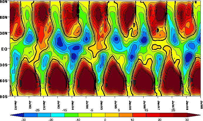 |
| Zonal mean wind as a function of time and latitude at 10mb |
- oscillation in mean zonal winds of the Equatorial stratosphere between easterlies and westerlies
- period of 28 months
- westerly shear zone propogates downwards more regularly and rapidly that easterly ones
-phase of the QBO affects the location of the extratropical surf zone by moving the zero wind line
- tropical mixing extent is dependent on the QBO phase
strong mixing extends to low latitudes of QBO pahse in stratosphere
Brewer-Dobson Circulation:
- large-scale middle atmospheric circulation
- responsible for long-term persistent transport of air and chemical nutrients from the troposphere to the stratosphere
- driven by Rossby wave breaking in the tropical stratosphere
Tropical Pipe:
- Tropical Pipe model of stratopsheric transport
- Tropical region bounded by subtropical edges of the wintertime surf zone which is isolated from the vigorous mixing of the extratropic surf zones
- edges of the Tropical Pipe barriers are moving
The seminar discussed the "influence of the stratospheric potential vorticity distribution in lateral mixing and transport into and out of the tropical pipe, th elow latitude ascending branch of the Brewer-Dobson circulation" and then presented the clear pattern that apparently exists between the above and the phase of QBO. I think the idea was that the phase of QBO dictates the amount of mixing that occurs as the phase of the QBO affects PV (potential vorticity) structure in the stratosphere. So, during the westerly phase, a strong PV is expected at the Equator which would isolate the Southerm Hemisphere from mixing and allow for greater 'in' mixing. During the easterly phase, stronger PV gradients at the subtropics limits Northern Hemisphere mixing and so particles remain in the tropics, where little mixing into the tropics occurs. I not quite sure if this is making any sense at all as I think the more I write about it the more confused I get about it all - therefore it is probably best that I just leave it at that! Sorry, I realise that my write-ups about the seminars have been really bad but honestly, they have all very quickly gone way past my level of understanding so, writing about the basics that they have been based on is about as much as I am currently able to manage.
Anyway, it was another great day and I hope Millie enjoyed it too!
Monday, 22 August 2011
Geography Picture of the Day - Formation of the Gulf Stream

I have spent some time this afternoon trying to create a way of representing the formation and journey of the Gulf Stream with minimal text. I am really bad at writing succintly so this has been a bit of a challenge and there is still way too much text on it, but I thought I would share it with you all anyway (any feedback on it would be great!) as I think, when it comes to the climate module, we do have to know a little bit about ocean circulation and this particular current, along with the North Atlantic Deep Water (NADW), play an influential role in moderating our climate.
Saturday, 20 August 2011
Inertia Currents
You may have got the impression from some of more recent blog posts that I have been spending quite a lot of my summer holidays trying to learn some of the basics of oceanography. Unfortunately, as our EPQ's can only be 5000 words long and have to be very specific, there are lots of interesting things, especially with regards to the thereotical side of physical oceanography, that I have to leave out. Instead I thought I would perhaps do a few more posts on here about some of the stuff I have been learning as, you never know, it may come in handy when we do the climate module as the oceans and atmosphere are very closely linked. So, first up is inertia currents........
There is, as with oceanography as a whole, an awful lot of maths involved with inertia current to calculate things like the centripetal force (which is essentially the Coriolis force in this case) so you can then move on to work out the period of the inertia current. I will spare you all the maths - I am currently staring at a bunch of equations that work this all out in a textbook and trust me it doesn't look very pleasant at all!!!
Anyway, apparently the equations demonstrate that, in an ideal situation, the only variable affecting the period of the inertia current (basically the time taken for a water parcel to complete one circuit) is latitude so, approximately, at latitude 45 degrees, it theorectically, the period of the inertia current is 17 hours whereas, at the Equator, it becomes infinite. Thats some of the theory, but these currents have actually be identified and observed in real life from the current measurements taken in many parts of the oceans. Here is an example of one observed in the Baltic Sea. The wind-driven current flowing to the north-north-west has been superimposed on by the inertial motion which, at this latitude, has a period of about 14 hours and, therefore, the inertia current died out after around 9 or 10 rotations.
So, I think thats about it really on inertia currents - I hope some of you found it interesting!
Winds are not always constant in strength or direction and so when a wind that has been driving a current ceases to provide sufficient energy to do so, inertia currents are created. Momentum will not leave the water immediately as, in open ocean, it takes a while to dissipate and whilst in motion, frictional forces and Coriolis force will continue to act upon them, thus resulting in a circular motion that characterises inertia currents. The extent of this circular motion is determined by the influence of Coriolis over other forces with the most circular inertia currents being generated when Coriolis is the only horizontally acting force on a current whose journey involves minimal latitudinal movement. The energy in the oceans is both kinetic, by virtue of its motion, and potential due to the displacement of isopycnic and isobaric surfaces and it is this huge store of potential energy in the oceans that ensures that the ocean circulation would take a few decades to completely cease if global winds stopped blowing.
 |
| Various possible paths for inertia currents |
 |
| Plan view demonstrating inertial motion in the Northern Hemisphere |
 |
| Plan view showing the inertial motion observed in the Baltic Sea |
Some external forcing factors with the ability to distrupt the general ocean circulation
As I have briefly discussed before, with reference to Heinrich events, the current ocean circulation pattern that exisits has not always do so and alterations to it in the past have resulted in huge shifts in the worlds climate. As well as those previously mentioned, there are some other external forcing factors that have the ability to affect the oceanic and atmospheric circulation. I think some of this stuff, like volcanic influence and Milankovich, comes up in the A2 syllabus although I don't know how much detail we go into - probably a bit more than I have done here, but hopefully the basics will still be useful!
 Volcanic eruptions, principally those that disperse ash and SO2 into the stratosphere which are most commonly high latitude (due to lower tropopause) explosive eruptions, can provoke a period of cooling that can last for a few years; like Pinatubo did after it erupted in 1991, releasing 20 million tonnes of SO2, cooling the Northern Hemisphere 0.5°C over 5 years. Despite their apparent ability to affect the climate, the effect they have on ocean circulation is debatable due to the variability produced by GCM. Some models show a connection between volcanic eruptions and a reduction in MOC intensity. However, these reductions appear to be small and short term and, this fact combined with other models not picking up the link above, suggest that the impacts of volcanic eruptions on ocean circulation, if there is one at all, is of little consequence and do not seem to pose a threat to the stability of the ocean circulation.

At varying points in time, external forcing factors have and will continue to provoke variability in the ocean circulation. Understanding them is, again, crucial as some explain the past changes that occurred, whilst others endorse future predictions.
 |
| There are two types of Precession: this diagram illustrates Axial Precession and this alters the hemispheric distribution of insolation. For more on Milankovich and the individual cycles see seperate blog post on The race for a million year old ice sample |
Many proxy-climate records suggest that the Milankovich ‘pacemaker’ has driven alterations in the oceans, atmosphere and the cryosphere; due to the moderation in the hemispheric distribution of insolation provoked by the three cycles, precession (23ka and 19ka), obliquity (41ka) and eccentricity (100ka). The spectral analysis of d18O variations present in marine carbonates over the last 10Ma, contain signals of all three cycles moderating high northern latitude insolation variations. Milankovich used this to explain the initiation and termination of ice ages and his theory states that the alterations in high-latitude insolation in the Northern Hemisphere are crucial in regulating the survival of snow through successive summers to warrant ice accumulation; a theory authenticated by the coincidence of glacial terminations and rapid increases in the solar insolation values of high latitudes in the Northern Hemisphere. The control Milankovich cycles exercise over hemispheric insolation distribution therefore dictates, although on a delayed timescale, the extension/shrinkage of ice masses (whether that be sea ice or ice-sheet/shelves) and it is because of this that they alter ocean circulation; although it is believed that precession has the largest influence. Generally speaking, the cycles range between two extremes, one favouring glaciation and the other deglaciation. When they favour glaciation, the THC is forced to downwell further south and thereby reduces northwards heat transfer and the associated ablation processes, to only further accelerate cooling. During glacial termination, the opposite is true and baseline increases in NADW intensity, beginning approximately 18ka, that parallel increasing Northern Hemisphere insolation, have been inferred from the RC11-83 South Atlantic Ocean floor sediment core. Many believe that it is the alterations provoked by this extrinsic forcing factor to the thermohaline circulation that drives, all atleast contributes, to the temperature changes that occur during transitions between glacial and interglacials.
Spectral analysis of variations of the chemical composition of ice cores have revealed that cycles shorter than those of Milankovich have occurred (periodicities of 11100, 6100 and 1470 years); with these sub-Milankovich cycles believed to be overtones generated within the climate system due to the influence longer cycles. The sub-Milankovich cycles can also be classed as an external forcing factor and can be attributed to shorter, abrupt alterations to the oceanic circulation. Precessional-driven climate alterations are believed to be linked to the 11100 year cyclicity which is being held responsible for temperature maximums being experienced every 11100ka in continents straddling the tropics. The 6100 year cyclicity seems to have a relationship with Heinrich events and other coolings such as the Little Ice Age and it is thought to only be amplified by ice-sheet presence. The shortest periodicity, because of the lethargic nature of ice-sheets, presumed to communicate readjustment of atmospheric circulation, is possibly due to solar output variations; something suggested by 14C records in tree-rings. When the sun is at its most ‘’energetic’, the Earth’s magnetic field is strengthened, blocking more cosmic rays. 14C is formed when cosmic rays hit plants, therefore measured in tree rings; with high levels of 14C suggesting an ‘inactive’ sun. Bond documented increases in icebergs and ice drift coinciding with the increase in 14C, indicating the sun was weaker at such times. Alterations in the volume of ice-rafted debris, in North Atlantic, also coincide with the 1470 year cyclicity, although are only 1/10 the size of the inconsistencies witnessed during the last glacial. Overall, there is agreement amongst scientists that these millennial-scale cycles, which have also been detected within ENSO, have a solar inception affiliated to the THC.
 Volcanic eruptions, principally those that disperse ash and SO2 into the stratosphere which are most commonly high latitude (due to lower tropopause) explosive eruptions, can provoke a period of cooling that can last for a few years; like Pinatubo did after it erupted in 1991, releasing 20 million tonnes of SO2, cooling the Northern Hemisphere 0.5°C over 5 years. Despite their apparent ability to affect the climate, the effect they have on ocean circulation is debatable due to the variability produced by GCM. Some models show a connection between volcanic eruptions and a reduction in MOC intensity. However, these reductions appear to be small and short term and, this fact combined with other models not picking up the link above, suggest that the impacts of volcanic eruptions on ocean circulation, if there is one at all, is of little consequence and do not seem to pose a threat to the stability of the ocean circulation.
 Sunday, 14 August 2011
Heinrich Events
 Heinrich events were first described in 1988 by the German marine geologist, Hartmut Heinrich, whose study demonstrated that six times during the last glacial huge iceberg armadas discharged from Canada into the North Atlantic, depositing, as they melted, lithic fragments. Peaks in the abundance of these lithic fragments far from land can only be attributed to icebergs melting as sea ice only transports dust and to further support this idea, much of the ice-rafted debris found consists of limestone similar to that exposed in much of Canada today (although lithic fragments from across the North Atlantic do feature). The lithic peaks form layers in sediment cores, known as Heinrich layers, which extend some 3000km across the North Atlantic, and seem to reflect an episodic nature in Heinrich events, with each one lasting approximately 1ka and occurring at intervals of 7-13ka (over the last 100ka).
 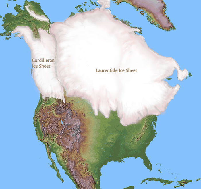 |
| Laurentide ice sheet during Last Glacial Maximum (LGM) |
The six events described by Heinrich are not unique as there are many lesser peaks in the lithic content of sediment cores. They are, however, the largest of the now recognised events in high-resolution core logs. In every event, icebergs were released when the surrounding surface water was cold but then abruptly warmed. All of this can be said with confidence but the exact cause of the periodic surges in the flow of the Laurentide ice-sheet (covered eastern Canada) provides an air of uncertainity as explaining the cause of the characteristic iceberg armadas is slightly harder than identifying them in sediment cores. There are, though, two fundamentally differing models that try to do this.
Denton model for iceberg armadas
The Denton model is essentially climatically driven as it based on global cooling leading to greater snowfall and thus a rapid expansion of ice-sheets/shelves and then marine ablation calving the icebergs from the expanding ice-shelf. Fundamentally the Denton model lays blame with the external cause of ice-sheet/shelf expansion as a result of global cooling as the forcing factor.
Advantages:-
- Evidence supports cooling in the North Atlantic before the Heinrich events
- The model explains the surging of South American glaciers and other global responses without the need for complicated teleconnections, during the same period of time
- Around 1.5ka climate cycles are known to have occured during the last 10ka and, despite them being an order of magnitude smaller than Dansgaard-Oeschger events, they too suggest external forcing over internal forcing
Disadvantages:-
- The model cannot explain the rapidity of events
- Heinrich events do not have consistent cyclicity as early on in the last glacial period they occured every 13ka but then later on they occured every 7ka
The MacAyeal 'binge-purge' model for iceberg armadas
 The MacAyeal ‘binge-purge’ model blames an internal cause (ice sheet failure) due to geothermal and frictional heat periodically building up and getting trapped beneath the ice-sheet, thus melting the base and provoking the catastrophic failure of the ice-sheet. So, instead of being climactically driven, it’s reliant on the mechanical failure of ice-sheets due to thermal modification at its base. MacAyeal suggested that the Laurentide ice-sheet grew whilst its base was frozen solid to both the crystalline rock (currently exposed on land in Canada) and the softer sediments found beneath Hudson Bay, to the south of the ice-sheet. When the base of the ice-sheet was heated enough, by geothermal heat, to cause the sediments to thaw, the rapid ice movement of the purge was initiated. Frictional heating then further increased the temperature, provoking a positive feedback as the ice movement was accelerated further. Despite this, the greater friction at the ice/crystalline rock meeting point prevented the total collapse of the ice sheet. This model highlights the fact that natural systems can display abrupt changes caused by a forcing factor that fails to change with time and so can occur independently of the external forcing factor; one of the reasons for the difficultly in making predictions about the future impacts of climatically driven forcing factors.
 Advantages:-
- The model is able to explain the rapid initiation and termination of Heinrich events - something that the Denton model fails to do
- Due to its dependency on the size of the ice sheet, it can explain the irregular cyclicity of Heinrich events
- Provides an explanation of the large amount of ice-rafted debris, which forms the Heinrich layer, found in the North Atlantic
Disadvantages:-
- Cannot explain the cooling known to have occured before each Heinrich event
- It needs a mechanism, such as the NADW, to transport the 'signal' around the world
Both models have their advantages and disadvantages and as a result there is a lack of consistency in which is favoured by scientists. For some time though, the 'binge-purge' model was favoured by most but then it was revealed that some of the Heinrich layers contained material that could have only came from other ice sheets, other than Laurentide. Attempts to generate a combined model have failed to paint a clearer picture of the mechanism provoking iceberg armadas but have led to further research into the conditions surrounding such events. Some of the sediment in the Heinrich layers has been linked to areas other than those covered by the Laurentide ice-sheet, such as Iceland due to basaltic glass fragments. This suggests that separate ice sheets surged simultaneously, something unlikely unless climatically driven or as a result of increased marine ablation due to eustatic sea-level rise thanks to Laurentide ice-sheet melt. The westward thickening of Heinrich layers, across the Atlantic, and its continuation towards Hudson Bay, point to the latter being correct and it is possible that its break-up triggered a response in other ice-sheets. Evidence insinuates that three gradual advances and rapid retreats of the Laurentide ice-sheet occurred towards the end of the last glacial, with glacial advances culminating before Heinrich events; thus provoking rapid ice discharge into the Atlantic, reducing southward ice flow and resulting in rapid retreat of LIS. There also appears to be synchronicity between the North Atlantic ice-rafting events and ice-sheet growth/ collapse in the Andes and New Zealand; something which supports the idea of strong inter-hemispheric coupling of changes in temperature and therefore global forcing of climate change. Research into the abundance of left-hand coiling in foraminiferid populations in ocean floor sediment cores, accompanied with studies into the origins of lithic sediments, have indicated that iceberg-calving events have occurred more frequently than first believed (intervals of 2-3ka), albeit on a smaller scale than the six originally identified Heinrich events. Of greater importance, is that many of the fragment peaks coincided with >90% proportions of left-hand coiling foraminiferid, thus revealing that the launching of iceberg armadas corresponded with low North Atlantic SST’s, symbolising stadial periods followed by the prompt warming leading into an interstadials. The use of d18O variations as a proxy record for eustatic sea-level rise and a lack of coherence between evidence of temperature rises in ice-cores from Greenland and Antarctica imply that meltwater discharge pulses, during the above events, originate from the Northern Hemisphere; an inference only endorsed by changes in salinity that are known to have occurred in the North Atlantic. As a result it can be said with confidence that Heinrich events influenced alterations in ocean circulation.
 There exists conflicting views regarding the influence of Heinrich events on THC. Some believe that the AMOC collapsed over the course of the six known Heinrich events, as a result of the influx of freshwater from glaciers interrupting the ‘normal’ circulation. Others suggest that NADW cessed as a result of each Heinrich event as the iceberg armadas placed a freshwater ‘lid’ over the northern North Atlantic. A Heinrich event is estimated to have provided a freshwater input in the order of 0.1Sv to the Atlantic, a volume believed to be sufficient to halt NADW formation, whose magnitude dictates the deep-ocean THC, and thereby explain the cooling observed in proxy data from the mid-latitude Atlantic. Some believe that Heinrich events were actually triggered by a reduction in NADW formation, due to freshwater fluxes to the North Atlantic as a result of the early deglaciation of the Fennoscandian ice-sheet. The reduced NADW formation would generate warmer SST’s, therefore perturb the ice-shelves, thus triggering iceberg armadas, allowing for the additional freshwater to further weaken, ultimately leading to the cessation of the MOC. Alternatively, several think that the collapse is relatively independent of the magnitude and origin of the freshwater input produced by Heinrich events, as long as it is transferred to North Atlantic convection sites; whilst events restricted to the Nordic Seas reduced NADW formation but didn’t provoke the cessation of the global conveyor; thus perhaps partially explaining the cause of Dansgaard-Oeschger events.
 This might seem a bit random, but I have just written up a section on the past changes that occured to the ocean circulation across glacial/interglacial and stadial/interstadial and so have mentioned Heinrich events, Dansgaard-Oeschger events and Bond cycles, amongst other things; unfortunately it is beyond the scope of my project to go into any real detail into the models used to suggest the causes of iceberg armadas and so, instead, I thought I would mention them on here. I have one question though, that I would be quite interested in knowing the answer to if anyone knows, what excatly caused the frequency of Heinrich events to change, from 13ka to 7ka, over the course of the last glacial?
Subscribe to:
Posts (Atom)