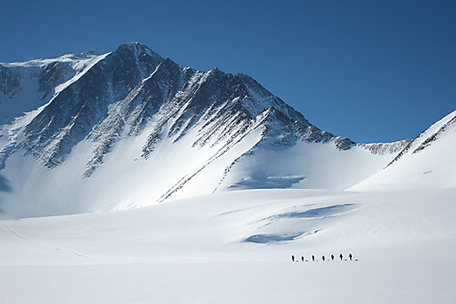
The first session I did was 'A virtual tour of Antarctica in 3D'. This involved us generating 3D images of the Antarctic Ice Sheet using GIS, in the form of ArcGIS, and data on the ice surface, ice velocity, surface temperature, bedrock and sea level - all of which had been collected from either satellite or field observations. Unfortunately I cannot show you the 3D images we made, so instead I am going to go through the facts, how the data we used was obtained and theory we were able to understand by making these images.
Antarctica is the major ice sheet in the southern hemisphere and the main ice sheet sits on the bedrock underneath - this is known as being grounded - and it was formed by snow falling on the land. The Antarctic ice sheet is different to the ice at the North Pole as this is floating sea ice (basically frozen sea water).
 |
| Highest Mountain = Vinson Massif, Ellsworth Mountains at 4897m |
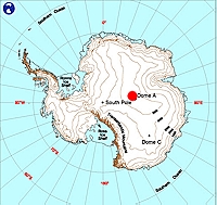 |
| Highest ice covered elevation = Dome A at 4090m Thickest ice = Around 4500m which can be found in East Antarctica Lowest point under ice sheet = Bentley subglacial trench which is around 2500m below sea level Coldest temperature ever recorded = -89.2 degrees Celcius at the Russian Vostok research station |
Ice Surface Elecvation:
This was the first data set we used and the measurements come from the use of an instrument, known as an altimeter, on board a satellite platform. The altimeter sends out either laser or radar pulses and measures the time taken for the signal to return. This measurement can then be converted into an elevation.
Bedrock underneath Antarctica:
As the ice is up to 4000m thick in most places, it is very difficult to measure the elevation bedrock beneath Antarctica. This means that a remote radar has to be used instead. The radar works as, as certain frequencies, ice is transparent to the radar and so this enables us kind of 'see through' the ice to the bedrock and therefore measure how deep it is beneath the ice. This factor is crucial if you are to understand ice flows in Antarctica as, because it is grounded, the bed below has a large influence on how the ice sheet flows.
Sea level:
Seeing as Antarctica is surrounded by ocean; knowing the ocean depth is really quite useful! This is measured either from a ship, or a satellite which take measurements of the sea surface, from which ocean depth can be inferred.
Ice free bedrock:
From the images we constructed we could see that a lot of the bedrock beneath Antarctice is below sea level which means the periphery of the ice sheet is susceptible to ocean warming - resulting in an increased melting rate. The rate of melt on the periphery is much higher than that on the surface due to the low air temperatures and so rises in ocean temperature are the largest threat to ice sheets.
Ice Shelves:
The images also showed up the location of ice shelves - areas of the ice sheet were the ice is not thick enough to float thus forms ice shelves - and the ocean cavities underneath them.
Ice Velocity:
Ice flows downhill, due to gravity, and radar instruments, on satellites, are used to measure how fast it flows (in metres per year). The pattern of flow in Antarctica is very complex due to the presence of both fast (the faster flowing parts are known as ice streams) and slow flowing parts - this is only made even more complicated by the fact that the ice sheet itself, which changes and thereby affects the flows, is an even more complicated system that it is extremely hard to predict. Despite this, it is important that the behaviour of these flows, inparticular their response to ocean and air temperature changes, are understood.
Surface Air Temperature:
The surface air temperatures are measured either from measurements on the ground or from satellites but the data we used, which was the annual mean temperature, was from the infrared measurements taken from the AVNHRR satellite. The images we produced showed how the temperature decreased with elevation, meaning that the interior of Antarctica is very very cold. This also means that it is only the periphery, in particular on the Antarctic Peninsula (the long thin part of Antarctica), of the ice sheet that experience a mean annual temperature that approaches 0 degrees Celcius.

The second session I did was 'The influence of plants and soils on current and future rates of climate change' followed by the 'Slartibartfast training programme'. Both these sessions heavily involved practical work and so I havent really got much to say apart from the things we learnt from the practicals.
The first part of this afternoon session was spent looking at the carbon cycle and the role that plants and soils play in the uptake of carbon dioxide - which is rather big! Neither of the experiments we did in this half of the session worked as well as they should of done but they, eventually, demonstrated the key trends they were intended to. Soils take up and release quite a bit of carbon dioxide and the rate at which they do so is influenced by climate. We measured the carbon dioxide changes in two different soil samples, one being kept at freezing point and the other at 31 degrees Celcius, and this clearly showed that the soil in the hotter conditions released much more carbon dioxide - from this we then discussed the likely impacts of global climate change on soils and why droughts lead to net carbon emissions often greater than the annual amount released from North America. Then we did another small experiment to show the difference in the amount of carbon dioxide when plants are able to photosynthesis and when they are not. If I am being honest I am not 100% sure what the point of this was apart from the fact that, accompanied by the change that occured in carbon dioxide concentration when someone breathed into the appartus, all living organisms are part of the carbon cycle. After this we moved on into the Experimental Lab which is just a huge room filled with complicated looking tanks and buckets and buckets full of various bits of sediment. We started off with the scaled down model of a river leading into an alluvial fan and looked out how changes in condition, especially an increase in erosion in the upper stream, changes the characteristics of an alluvial fan which is not a static landform and so shouldnt really be built on - although many do! After looking at that we moved to the other, and rather wet end, of the room to look at the differences in the rate of erosion depending on the location of the strip of exposed soil, in this huge soil bed, that is exposed to the rain - when I say rain I literally mean that they have these pipes in the ceiling which, when turned on, generate rather a lot of rainfall! This also demonstrated the non-linear relationship between the depth of the water and the erosion and transportation of sediment.
Well apart from talks about applying and going to Exeter University, that is what me and a few others got up to today. It was quite an intersting day but unfortunately, without seeing the things I did for yourself, its hard to understand it or actually really gain much from it - so, apart from saying thanks to Nick for taking us up their today, that its from me tonight.
No comments:
Post a Comment